
In the previous post, we began to build a theory of detection over time as the result of a very large number of independent glimpses. By assuming the environment to be fixed for awhile, we moved all the environmental factors into a constant (to be measured and tabulated), and simplified the function so it depended only on the range to the target.
In this post we simplify still further, introducing lateral range curves and the sweep width (also known as effective sweep width). We will follow Washburn's Search & Detection, Chapter 2. (So there's nothing new in this post. Just hopefully a clear and accessible presentation.)
Detection Rates, Randomness, Tests
The model we developed in the last post is a detection rate model. Instead of searching for a single object, imagine you were in a target-rich environment. Then if each glimpse had the infinitesimal detection rate 

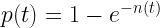
Then our probability of detection from the previous post becomes:
Washburn notes that as long as detections are independent, the actual number of detections N(t) has a Poisson distribution (that's what you get when events are independent), which has n(t) as the expected value (average).
Why should we care? For one, because it's a testable prediction for a controlled experiment! Washburn says,
The reader should note that in deriving [detection probability and expected time to find], we have at no time given any instructions as to how such a search could actually be carried out.... The real justification is ... the fact that those formulas provide good approximations in a wide variety of circumstances.
In a sense this is surprising. As both Washburn and Koopman note, the independence assumption amounts to cutting our actual, sensible search track into confetti, and scattering the confetti across the search area. The confetti overlaps. No one searches this way. No one should. So how can the model possible work?
- Real detection functions are never 100% to begin with.
- Imperfect navigation means our sensible planned tracks actually do overlap in unplanned ways. Not quite like scattering confetti, but with similar effect.
- Even a little target motion means that in the target's coordinate system, our sensible search plan starts to look random.
Washburn then cites experiments with pursuit-evader games run on a computer using ideal "cookie-cutter" detection functions. Even there, the results agree remarkably well with random detection. The evasion introduces deviations that drive the detection curve down to the random search model.
So we will confidently adopt a random detection model. But how do we estimate the detection rate 
We don't.
Lateral Range and Sweep Width
In most cases where the target is not trying to evade us, we can model our search as a straight track past our target: the closest point of approach is the lateral range. Many sensors can simply be characterized by their lateral range curve. And if operational noise drives us down towards the random detection model, it isn't even necessary to know the shape of the lateral range curve -- all we need is the area under the curve, known as the sweep width.
Lateral Range Curves
Suppose you can write down your detection rate as a function of range, as with Koopman's inverse cube law from the previous post. In that case, you can get your total probability of detection by integrating along the line. A very useful case is to imagine a hypothetical straight track from horizon to horizon, passing the target at minimum distance x, the lateral range.
 The total probability of detection is the integral along that line, from horizon to horizon. Your
But if we calculated (or measured) this probability for lots of values of x, you would generate a lateral range curve, showing how your total probability of detection dropped off with the lateral range of your search track.
Important! Each point on the lateral range curve is the detection probability for a whole search track. It's not the glimpse detection probability for being x meters away! The glimpse probabilities are much smaller.
These curves can have many shapes. The following figure shows four lateral range curves with central peaks. All four have the same area as the blue rectangle.

Any given sensor (in a given environment, for a given target) will have a lateral range curve that describes its performance as a function of lateral range. (It may or may not have a central peak.)
In good conditions, search planners should consider the actual shape of the lateral range curve when planning searches. However, as we have seen, in many cases there is unavoidable overlap (at least in the target's frame of reference), meaning that we lose the benefit of careful planning. In those conditions, the only property of the lateral range curve that matters is the area under the curve.
Sweep Width
The area under the curve is called the sweep width, or effective sweep width (ESW), often written simply W. Because W adds up the detections at various lateral ranges, it tells us the expected number of targets we would detect in a single track through a large field containing many randomly placed targets.
Because these four sensors have the same sweep width, they have the same detection rate. Therefore, on a single pass, they would be expected to find the same total number of targets. The cookie-cutter sensor would find all the targets within 10m of either side of the path, and none outside. The triangular sensor would find half of the targets out to 20m on either side of the path, in decreasing proportion (so that it found 75% of those within 10m and 25% of those between 10m and 20m). The inverse-cube sensor would miss more up close, but find many quite far out, and the Gaussian would be somewhere in between. The effective sweep width W is 20m, the actual width of the (equivalent) cookie-cutter.
But what about multiple tracks? If we keep good parallel lines, the equivalence vanishes. In a perfect world, you can't beat a nice cookie. Multiple cookie cutters spaced W apart make a clean sweep with no overlap, so the search region's cumulative probability of detection rises linearly from 0% to 100%.
No other sensor can do that, but we can space them optimally for their own lateral range curve, and get performance substantially better than the random detection curve. The following image shows the range of variation.

In the common case where various factors conspire to introduce uncontrolled overlap, all sensors are driven to the random detection curve, making it a good conservative model for actual performance. On the random curve, only W matters.
Next: sweep width and (average) maximum detection range
Thanks to Ken Chiacchia for suggesting I use the full lateral range curves. Post updated silently. (Almost.)
Q: But trained searchers work as a team, maintaining their separation. Shouldn't we use a different model for teams?
A: Yes, if they maintain good spacing, then ideally we should use the math for proper parallel tracks (or just measure them as a ganged sensor platform to begin with). Washburn and others cover that too.