We begin a four-part gentle introduction to search theory. Our topic is visual detection of targets by land searchers. Today we summarize Koopman Chapter 3, constructing the useful "inverse cube" detection model by starting from instantaneous glimpses with tiny detection probabilities.
It All Starts with Glimpses
Way before we get to POA and POD, we have glimpses -- the smallest unit of detection. Glimpses are the building blocks of search theory. Koopman modeled visual search as a series glimpses. Detection can happen on any glimpse, and importantly, the glimpses are assumed independent: failure on one attempt does not alter the chances that the second will succeed.
This independence assumption means that the overall probability of detection (POD) that we model is the average result integrated over all glimpses as a searcher approaches and passes a target. (In land search, the target is either the subject, or a clue.) The detection probability on an individual glimpse is quite small, but there are many glimpses.
The assumption of independence is false, but not fatally so. It's false because some targets are obscured, buried, or otherwise hard to see, compared to an exact duplicate that is just laying on the grass. Therefore continued failure to detect makes it more likely that any clues present are "hard cases", and so the detection probability drops. However, we can ignore this if we consider conditional detection probabilities, such as the probability of detection given the clue type and environmental conditions, or measure our probabilities for some average condition.
Instantaneous Detection Probabilities and Expected Find Time
This is pretty cool, even if you skip the math. It shows how clear thinking can take you from basic glimpses to probabilities of detection.
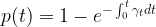
We begin with g, the instantaneous probability of detection in one glimpse. Because we assume that glimpses are independent, we have what is known as a Bernoulli trial, which means it's like a coin toss: the failures multiply. The chance of getting a head (detection) on n tosses (glimpses) is one minus the chance of getting no heads (missing the target on all n glimpses). That means the the overall probability of detection 

The expected number of glimpses until detection can be shown to be 
We might use this discrete glimpse approach for a computer simulation. But in general it's more helpful to assume looking is continuous (i.e. that glimpses are really small). In the case of continuous looking, the analog to g is the probability of detecting in a very short interval of time dt. We denote that probability as 


and the expected time to detection is 
Notice we're happily humming along without having a clue about the values of g and
Accounting for Searcher Motion
The previous model assumed a constant g or
Therefore we have to add up our glimpses as 
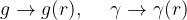
But it's not really time that matters: g and
Now Koopman uses insight or intuition to help solve the equation. He assumes the environmental factors would be roughly constant for a given scenario, and so could be measured and made into tables. That leaves only the range r:
The Inverse Cube Model
By assuming (quite reasonably) that

This is the famed "inverse cube" law of visual detection. Although derived for aircraft searching over water, it has been shown to apply in a great number of circumstances, leading Washburn to quip that it "may be holy''. In practice it is often modified for particular conditions, to account for the way the eye works, but it is considered "a remarkably useful approximation''.
However, it is worth noting that the good results in WWII were obtained using the solid angle of the wake. Koopman writes:
Further, if the solid angle is that subtended by the actual solid hull of the target, perfectly tractable mathematical formulas are obtained, but they give results inconsistent with the operational data on surfaced submarine sightings of World War II. This confirms the experience of naval aviators that the most visible feature of surfaced craft is the wake rather than the hull. (p.59)
Koopman's experience reminds us of the need for experiment. Alas, there is likely no analog to the wake for most clues or missing persons, so we would have to use the smaller size of the target.
Alas again! As we will see in the next post, there is now reason to think the inverse cube law is a poor model for dismounted land search. That does not invalidate the theory, only this particular choice of
As an aside here, Koopman notes that in general, the actual probability of detection will depend upon the line integral of relative motion of the searcher and target. But the model is now complicated enough. When the searcher and target are on straight courses at constant speeds for a long time before and after their closest approach, the probability of detection is simply a function of the lateral range x at the point of closest approach. We consider this a good model for non-evasive subjects. It is of course an excellent model for stationary subjects.
I would be honored to hear some of your search techniques or read some of your pdf files on search techniques.
Thanks James. If by techniques you mean something like a style of mantracking, I don't have anything to say. A given technique will have a given detection profile for a given target, environment, and search speed, assuming the technique is applied correctly by someone with expertise. Once those are measured, an optimal plan can be developed.
Certain tactics do fall out of theory. Absent GPS tracks, we're necessarily only concerned with total effort in a search segment, and must assume that effort is spread out, or at worst scattered randomly. But in repeated searches through a wilderness area, teams will wear down paths, which will attract following teams, potentially leading 3 teams to follow nearly identical paths -- highly suboptimal. So a simple tactic is to send subsequent teams in at right angles or at least substantial angles relative to each other.
A very interesting area I wish I time to think about is treating the team as a single sensor. I think that approach more closely matches wilderness SAR practice.